Calculating Time-to-First-Fix

By Nicolas Couronneau, Peter J. Duffett-Smith, and Alexander Mitelman

Cell-phone users are often more concerned about the speed of positioning than the accuracy, making time-to-first-fix the most important factor in a GNSS mass-market receiver’s perceived performance. However, TTFF is generally difficult to characterize and optimize because of the need to encompass a wide range of environments, including indoors.

One method of characterizing the time-to-first-fix (TTFF) is to measure it directly, using a signal generator and a real receiver. This method avoids the approximations of analytical solutions, but it is usually time consuming and it does not provide much insight into the factors affecting the TTFF since it is gen erally not possible to change the receiver’s architecture. Another approach is to use Monte Carlo simulations and a model of the acquisition process. This approach is more flexible than direct measurement, but again it can take a long time to simulate weak-signal environments.

We have developed a third approach based on analytical methods but regulated by measurements of the signal-to-noise ratio in target environments. Using this approach, one can quickly calculate the probability distribution of the TTFF for different signal strengths and acquisition parameters.

To illustrate this method, we consider a model of an assisted-GPS receiver combined with experimental measurements of the GPS L1 C/A signal taken indoors. The results are presented in Figure 1, where the probability of the TTFF (horizontal axis) is plotted as a function of the time after the beginning of the data series at which the acquisition process started (vertical axis), calculated using a 400-second GPS data series measured indoors. The strength of our approach is that we can quickly calculate the TTFF probability for any given confidence level and it is quite general so that it can be extended to other types of receivers.

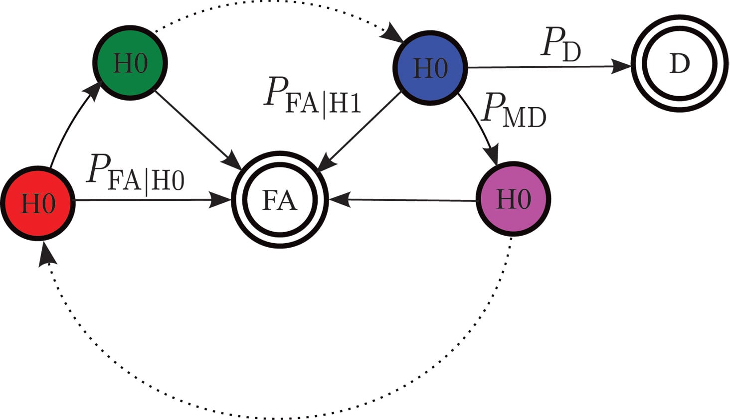
Flow-graph representation of the acquisition process for one channel. FA is the false-alarm state and D the correct detection of the signal from this satellite. H1 and H0 represent respectively states in which the signal is and is not present. PFA|H1 is the probability of false alarm in a window where the signal is present and PFA|H0 the probability of false alarm in a window where the signal is not present. P D is the probability of detection, and PMD the probability of missed detection.

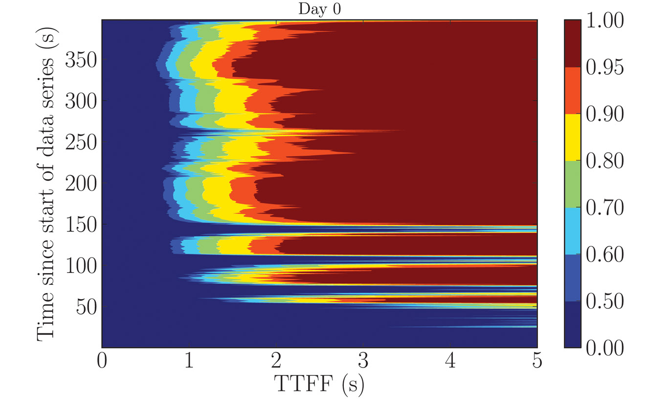
Figure 1. The probability of the TTFF (horizontal axis) as a function of the time after the beginning of the data series at which the acquisition process started (vertical axis), calculated using a 400-second GPS data series measured indoors. Note that the colored scale is not linear.

Modeling the Acquisition Process

A GPS receiver must first acquire signals from a sufficient number of satellites before it is able to calculate a position. This search is often the major contributor to the TTFF.

GPS Acquisition Architecture. The acquisition can be represented as the search for a specific, yet unknown, combination of three parameters in a larger search space. These are:

• the Gold-code number used to generate the pseudo-random noise (PRN) sequence,
• the code phase, and
• the carrier frequency offset.

The last of these has contributions from the frequency offset caused by the relative motion of the satellite and receiver (the Doppler effect) and the frequency bias of the receiver’s local oscillator.

In general, signal detection is performed by correlating incoming signals with a local satellite signal replica for every combination of parameters in the search space. The correlated signal is then integrated and a “hit” is declared if the integrated value crosses a predetermined threshold. The time required to test for the presence of a satellite signal for each combination of parameters is called the dwell time. We suppose here that this is approximately equal to the integration time.

GPS receivers usually include some degree of parallelism. We consider a receiver having N channels, each channel dedicated to searching for signals with a different PRN sequence. Within a channel, the frequency and code-phase search spaces are further divided into several windows. We assume that all the parameter combinations within a window are searched in parallel, that is, within a single dwell time. This model of the acquisition process is outlined graphically in Figure 2.

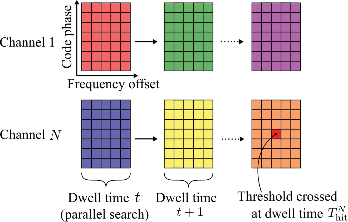
Figure 2. An illustration of the acquisition process. The large colored rectangles represent the search windows and the inner smaller rectangles represent the different combinations of search parameters.

Parallelism can be implemented in hardware using massively parallel correlators or in software using fast Fourier transform-based techniques. The details of any particular implementation are not relevant here; only the number of channels, the number of windows, and the sizes of the global search spaces are needed.

Acquisition Time Probability Distribution. The flow-graph method provides a graphical representation of the acquisition process. An example is shown in the Opening Figure. Each node represents a state of the acquisition process at the end of a dwell time. The lines joining the nodes represent the transitions of one state to another with the given probabilities. Typical states during acquisition are false alarm, missed detection, correct detection, and correct non-detection.

The flow-graph method has already been applied to the GNSS acquisition problem, in particular for calculating the mean acquisition time of a signal in a GNSS receiver. Here we extend that work by considering the acquisition of all the satellites required for a position fix and, by deriving full probability distributions, we establish a model of an assisted-GNSS receiver.

The opening figure shows the various probabilities of transition that can be calculated from detector statistics.

Flow-graphs rely on the properties of the probability generating function (PGF) of a random variable. A PGF makes it straightforward to calculate the probability distribution of the total duration of a sequence of events of random durations since the PGF of the sum of random variables is simply the product of their PGFs. It is also straightforward to calculate the mean and standard deviation of a random variable directly from its probability-generating function.

Aside from these properties, PGFs are less convenient and less intuitive than probability distribution functions. A generating function does not provide a direct calculation of the probability of an event, unlike a distribution function. For instance, calculating the acquisition time at an arbitrary confidence level (for example, 90 percentile) requires a contour integral over the PGF. Furthermore, some operations are easier to perform on density functions, for example, calculating the probability of simultaneous events.

It can be shown that the probability mass function of a discrete random variable can be approximated from its generating function using a discrete Fourier transform. This property forms the basis of our method: using the fast Fourier transform (FFT), we can quickly calculate the entire acquisition probability distribution associated with the generating function of a flow-graph.

Assisted-GPS Model

We now focus on the specific architecture of an assisted-GPS receiver, such as is commonly found in cellular phones. In this type of receiver, the TTFF can be shortened by performing the acquisition in two steps.

The acquisition starts by searching for any satellite signal in a full search space in which every parameter takes its full range of values. The Doppler frequency of the first satellite acquired can be calculated using assistance data and then removed from the observed frequency offset to give the contribution to the frequency offset caused by the receiver’s clock frequency offset. This is common to all search channels and can be removed from the remaining search spaces.

The second stage of the acquisition is thus performed for the remaining satellites over a reduced search space.

Stage 1 Full Search Space. The first threshold crossing for a single satellite is characterized by the time-to-first-hit (TTFH). Using an FFT, we can calculate the distribution function P(T_hit^full ⩽ t) of the time-to-first-hit T_hit(k) of the k^th channel.

Mathematically, the time to first hit across all N channels, T_hit^full, is the minimum of {T_hit(k)}, whose distribution function is calculated by:

We assume that we have no means of detecting a false alarm at this stage and so the frequency parameter of the first threshold crossing is used to calculate the receiver’s clock frequency offset. This crossing may, of course, be a false alarm, and we take this into account later.

Stage 2 Reduced Search Space. At the reduced-space stage, the goal is to calculate the probability of having acquired M satellites out of N channels. The value of M depends on the number of pseudorange observables needed to solve the position equation. High-sensitivity assisted receivers that do not have signal tracking loops can only measure fractional pseudoranges together with an uncertain number of integer code periods. Using a coarse position estimate of the receiver, this uncertainty can be resolved, and a 3D position fix obtained, by using M = 5 satellites.

Calculating the detection probabilities at this stage involves some combinatorial arguments. In the following, (^Ω_m) represents the set of all combinations of m elements from the set Ω. For example, if Ω = {a, b, c}, then (^Ω₂ ) = {{a,b}, {b,c}, {a,c}}.

The probability of having “hit” at least M signals out of N channels at time t is given by

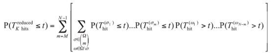
In this equation, Ω = {1, …, N} represents the set of the receiver’s channels and T_hit(k) is the time to first hit of satellite k. Because each satellite is received with a different signal strength, these random variables have different distributions for every satellite.

The probability of having correctly detected at least M satellites before time t, P(T_D^reduced ⩽ t), is calculated by enumerating all the possible combinations of hit and detection events. The probability of having at least one false alarm before a given time t, P(T_FA^reduced⩽ t), is simply calculated by taking the difference between the probability of a hit and the probability of detection.

The number of possible combinations grows quickly with the number of channels. For an 8-channel receiver, there are 35 combinations, and for a 24-channel receiver there are 8,855 combinations. If the number of summations is becoming too computationally demanding, one solution is to form sets of signals with similar strength, and perform the combinations over these smaller sets with an appropriate weighting. Within a smaller set, all the signals have the same signal strength and acquisition times have the same probability distributions — a situation that is similar to calculating the order statistics of a random variable, which is not problematic in the case of identical distributions.

TTFF Probability Distribution

The last step before obtaining an expression for the TTFF distribution is to combine the two stages of the assisted acquisition. The total acquisition time is the sum of the time to first hit in the full-space stage and the time to the correct detection of M satellites in the reduced-space stage. This sum is easily calculated using generating functions, with the corresponding flow-graph represented in Figure 3.

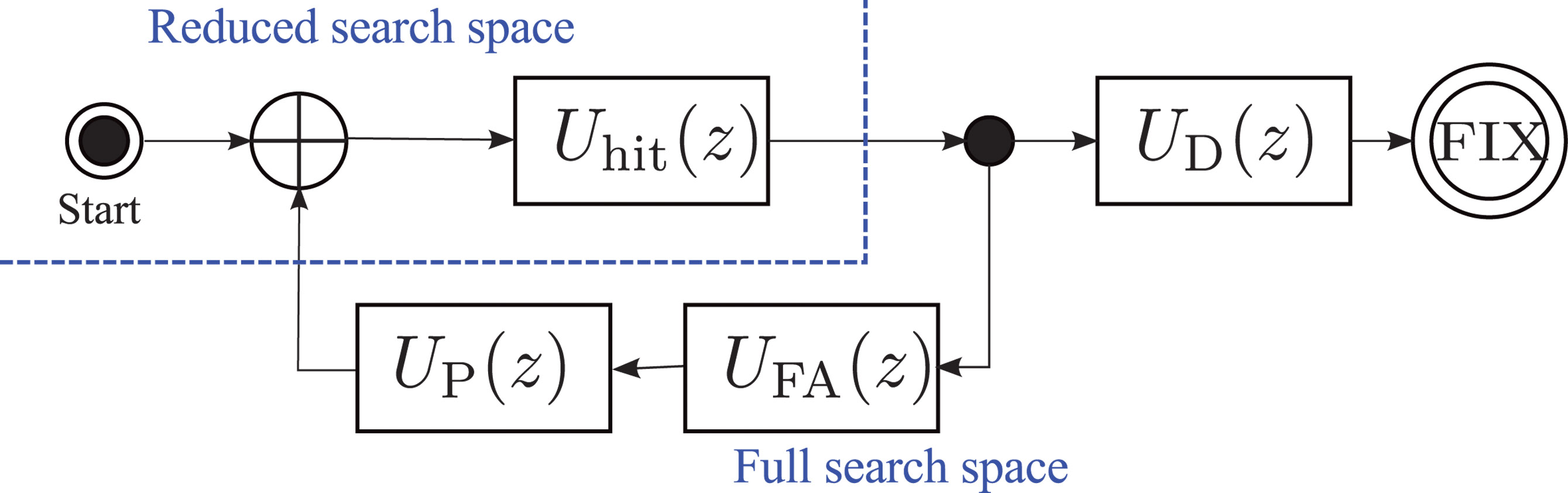
Figure 3. Overall flow-graph of an assisted receiver. Uhit(z), UD(z), UFA(z), and UP(z) are the generating functions of the time to first hit in the full-space stage, the time to detections in the reduced-space stage, the time to a false alarm in the reduced-space stage, and the penalty time to recover from a false alarm, respectively.

Using the inverse of the FFT method presented above, we calculate the generating functions of the time to first hit in the full-space stage, U_hit(z); the time to M detections in the reduced-space stage, U_D(z); the time to a false alarm in the reduced-space stage,U_FA(z), and the deterministic time penalty to recover from a false alarm,U_P(z).

Modeling false-alarms demands special attention. There is little information in the literature about the detection of false alarms in assisted-GPS receivers. One solution could be to detect a large residual error at the output of the positioning algorithm. Here, we take an easy path and simply introduce a penalty time, T_Penalty, to represent the (deterministic) time needed to recover from a false alarm. The penalty time should be chosen to represent the behavior of a specific receiver.

For GNSS receivers capable of tracking the signals, the full pseudorange can be recovered after detection of a synchronization word in the navigation message. The duration of the tracking stage is a random variable, since the tracking can start at any position in the navigation message. Although we have not investigated this situation in more detail, we suspect that the tracking stage can be simply modeled by a uniform probability distribution. The length of this distribution depends on the navigation message structure and the amount of navigation data needed by the receiver to obtain a full set of decoded data. A new block can be added to the flow-graph in Figure 3 using the generating function of the uniform distribution, and the TTFF for a standard GNSS receiver can then be calculated.

Experimental Results

We analyzed the TTFF with the signal strengths measured in an office environment.

A picture of the office is shown in Figure 4. One side of this office has a window, but the sky view is obstructed by a large building a few tens of meters away. There is no direct line of sight to a satellite, although the window may allow some strong reflected signals to get in to the office.

Measurement of Weak Signals. Direct measurement of the strengths of indoor signals can be challenging since the signals are often too weak to be tracked reliably. We used a Nordnav R30 dual-input receiver with one input connected to an outdoor antenna mounted on the roof of the building and having an unobstructed view of the sky. The other input was connected to an antenna in the office. We used the tracking information from the stronger outside signal to track the indoor signal.

The signal carrier-to-noise density ratio (C/N₀) was recorded for 400 seconds, starting every day at the same sidereal time, for six consecutive days.

Figure 5 shows the signal strength for one particular satellite (GPS PRN9). We see that the signal strength follows a similar pattern every day. This is representative of a multipath fading environment: the signal coming from the satellite is scattered in the office, and the resulting signals interfere constructively or destructively, depending on the phase difference between the different paths. The overall signal strength is therefore related to the relative position of the satellite which, for GPS, is about the same every day at a given sidereal time.

The variations of the signal strengths of all the observable satellites show fading patterns which are uncorrelated, as we expect the satellites to be spread across the sky (see Figure 6). It is difficult, if not impossible, to predict the distribution of signal strengths at any specific instant, and so the TTFF varies depending on the instant at which the acquisition process begins.

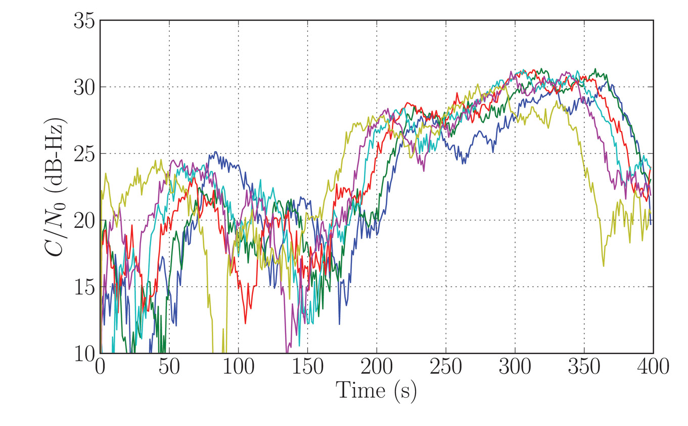
Figure 5. Indoors signal strength (C/N0) for satellite PRN09. Each colored curve represents the signal strength measured on a different day, starting at the same orbital time.

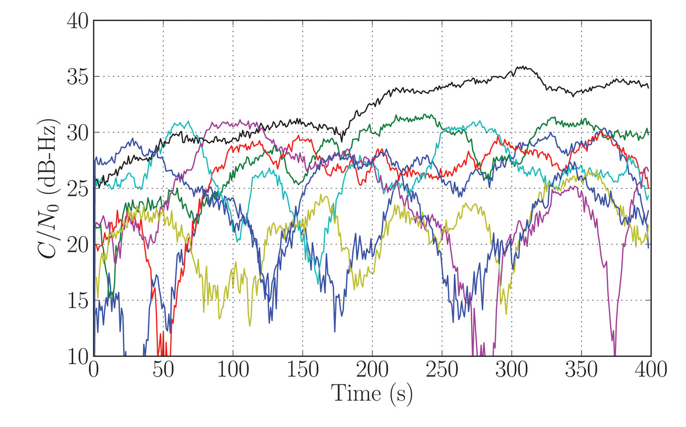
Figure 6. Measured C/N0 for all observed satellites during the first day of recording.

TTFF Indoors. We now apply the signal strength measurements (Figures 5 and 6) to the TTFF calculation method presented above. This allows us to determine the probability of the TTFF as a function of the starting time of the acquisition since the beginning of the data recording.

We chose the detection parameters as follows: the coherent integration time was 1 millisecond, the non-coherent integration time was 300 milliseconds, the threshold was set for a probability of false alarm of 10^–6, the time offset of a code phase was between 0 and 1 milliseconds, the penalty time for a false alarm was set to 600 milliseconds, and five satellites were required to solve the position equation. The ephemeris, a coarse position within 150 kilometers of the true position, and a coarse time within 30 seconds of the GPS system time were provided by the assistance data.

The results (see Figure 1) provide some insight into the acquisition process.

We can discern two patterns in the TTFF distribution. During the first 150 seconds of the analysis, that is, if a real receiver had started acquisition during that time, the TTFF showed large variations. This was caused by the multipath. The fading of the signals from the various satellites, although uncorrelated, led to severe degradation of the TTFF when the acquisition was started during a combination of strong fades. In our analysis, we have made the simplifying assumption that the strength of any particular satellite signal remains constant over the acquisition period.

After the first 150 seconds, the TTFF became more nearly constant. On examining the C/N₀ time series, it was clear that the reason was the appearance of a signal from the satellite with PRN 27 (black curve in Figure 6) which was consistently stronger than the remaining signals after 120 seconds. This satellite had the highest elevation (more than 60 degrees) and the reception was probably by transmission through the ceiling of the office. In this situation, the phase difference between the reception paths was small, hence there was little fading. This single satellite significantly improved the TTFF, in particular by shortening the time of the first stage of the assisted-acquisition process.

It can be shown that the distribution of the acquisition time of a satellite, at a given starting time, can be approximated by an exponential distribution. This distribution explains the non-linearity of the relationship between the TTFF and the probability of fix, as observed in Figure 1. The non-linear effect becomes important when calculating the TTFF at a given performance level. In our example, the 50-percent probability of fix was about 1.2 seconds. Moving the requirement to 90 percent made it about 2 seconds, and 95 pecent about 2.5 seconds.

Conclusions

In presenting a method of calculating the distribution of the TTFF representative of a mass-market receiver indoors, we have seen how existing techniques can be extended and combined to provide an analytical model for assisted receivers. Power measurements of real signal show how the TTFF can vary depending on the combination of signal strength at the time the acquisition process is started. This suggests that an improved strategy for acquisition in large search spaces might be to start two or more independent acquisition processes, separated by, say, 1 second, in order to benefit from the advantage of one of the signals appearing strongly after a fade.

The lead author gratefully acknowledges support for this research from Cambridge Silicon Radio, CSR plc.

Nicolas Couronneau is a Ph.D. student at the Cavendish Laboratory, University of Cambridge, UK. He graduated as an electrical engineer from Supélec, France. His research interests are in the area of probabilistic methods applied to the acquisition of GNSS signals.

Peter J. DufFett-Smith is reader in experimental radio physics at the Cavendish Laboratory. His Ph.D. was in radio astronomy. He is the founder of Cambridge Positioning Systems Ltd. and, with others, invented the Matrix positioning method and Enhanced-GPS technologies. He holds more than 20 patents, and is a consultant to the GPS Group at Cambridge Silicon Radio.

Alexander Mitelman received his Ph.D. degree from Stanford University in electrical engineering. His research interests include signal-quality monitoring, algorithm and system design, and the development of testing methodologies for GNSS and hybrid systems.