
GPS accuracy: Lies, damn lies and statistics

EDITOR’S NOTE: An updated version of this article appeared as our January 2007 cover story.
Frank van Diggelen, Ashtech, Inc.
“There are three kinds of lies: lies, damn lies, and statistics.” So reportedly said Benjamin Disraeli, prime minister of Great Britain from 1874 to 1880. And just as the notoriously wily statesman noted, the science of analyzing data, or statistics, sometimes yields results that one can interpret in a variety of ways, depending on politics or interests. Likewise, we in the satellite navigation field interpret results depending on the information we wish to produce: Using various statistical methods, we can create many different GPS and GLONASS position accuracy measures. It can seem confusing, even misleading, but as we’ll see in this month’s column, there’s some rhyme to our reason. We’ll examine some of the most commonly used accuracy measures, reveal their relationships to one another, and correct several common misconceptions about accuracy. Our author is Frank van Diggelen of Ashtech, Inc., in Sunnyvale, California. Van Diggelen is the OEM (original equipment manufacturer) and navigation products marketing manager.
“Innovation” is a regular column featuring discussions about recent advances in GPS technology and its applications as well as the fundamentals of GPS positioning. The column is coordinated by Richard Langley of the Department of Geodesy and Geomatics Engineering at the University of New Brunswick, who appreciates receiving your comments as well as topic suggestions for future columns.
Root mean square (rms), twice the distance root mean square (2drms), circular error probable (CEP), spherical error probable (SEP), so on, and so forth — Why do we have so many different position accuracy measures? The answer lies in the fact that the errors of position coordinates determined using a GPS or GLONASS unit are not constant — they vary statistically. If you observe the reported position of a stationary receiving system over time, you will notice it wanders. Graphing these moving points yields a “scatter plot”; how you analyze the scatter depends on the information you want to obtain. To complicate matters, the position is fundamentally three dimensional, but not everyone is interested in obtaining three-dimensional accuracy. One user might care about horizontal accuracy, another might want vertical. Thus, clearly, we must consider different accuracy measures.
Before we take a look at some of the common accuracy evaluations and their relationships to one another, we must say a word about the meaning of accuracy itself. To ascertain how accurately a system has determined a point’s coordinates, you must know the point’s true coordinates. Typically, this comes from measurements made using a system with an inherently higher accuracy than the one being tested. Simply averaging a system’s reported positions will provide an indication of system precision or repeatability, but the measurements might contain a bias that could affect the results. So, when we talk about system accuracy, we must consider the possibility of such a mean error.
POPULAR ACCURACY MEASURES
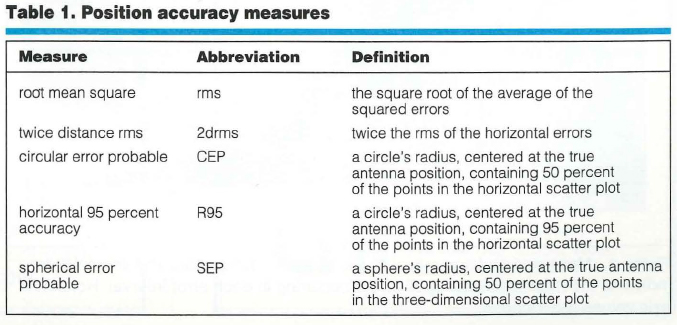
Table 1 lists the most commonly used GPS position accuracy measures and their definitions. Note that the first two methods are explained in terms of average squared error, and the last three are defined directly from the position error distribution (the scatter). Thus, we can immediately associate these last three with error probabilities. If we assume that the error distribution along any axis (east, north, or up) is “normal” or Gaussian, then we can also derive probabilities associated with the rms and 2drms accuracy measures. [The normal or Gaussian distribution is the one to which the dispersion of the sum of a very large number of very small errors always converges. The famous German polymath Carl Friedrich Gauss used this distribution to develop his error theory in the early nineteenth century. To honor the importance of this and the scientist’s other accomplishments, Germany features a portrait of Gauss and his probability distribution on its 10-mark bank note. — R.B.L.]
Data: Frank van Diggelen
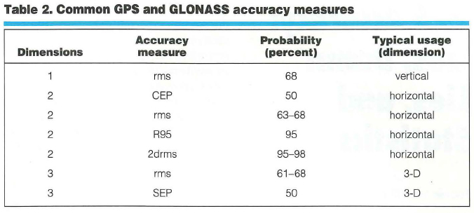
Table 2 shows how the accuracy measures are used and what probabilities can be associated with them. Note that the probability associated with rms depends on whether one is using rms in one, two, or three dimensions (1-D, 2-D, or 3-D). The later “Common Misconceptions” section discusses this further.
Data: Frank van Diggelen
Ascertaining Accuracy: An Example. Now, suppose you are comparing the specifications of two positioning systems. One unit has a quoted accuracy of 3 meters (3-D rms) and another has a quoted accuracy of 2 meters (CEP). Which system is more accurate?
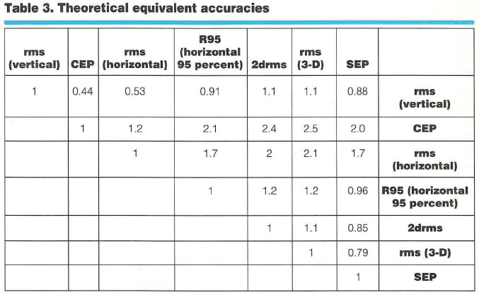
By making three assumptions about the ratio of east, north, and up errors, we can relate different accuracy determinations to each other, as shown in Table 3 (entitled “Theoretical Equivalent Accuracies”).To use that table, identify the desired measure in the top row and the original measure in the right hand column. Take the number in the cell at which the row and column intersect and multiply it by the original measure value to yield the desired number.
Data: Frank van Diggelen
The three assumptions, from which the conversion values derive, are true on average. First assumption, the error distribution is Gaussian. Second, the ratios of the position dilution of precision (PDOP) to the horizontal DOP (HDOP) and the vertical DOP (VDOP) to the HDOP are 2.1:1 and 1.9:1, respectively. Third, the horizontal error distribution is circular. These suppositions are based on simulations performed over a grid covering the entire globe between latitudes 66 degrees south and 66 degrees north. In general, horizontal distributions are elliptical, the ellipses are often very close to circular, and the circular Gaussian distribution model is very good at estimating the true distribution, as shown in Figure 1.
To answer the question posed earlier (which is more accurate — a 2-meter [CEP] or a 3-meter [3-D rms] system?), follow these four steps:
- Go down the “rms (3-D)” column to the “CEP” row.
- The entry in this cell is 2.5.
- According to the table, rms (3-D) =2.5 3 CEP.
- So, CEP = rms (3-D)/2.5 = 3/2.5 =1.2 meters.
Thus, a system with 3-D rms of 3 meters will have a CEP of 1.2 meters and is, therefore, more accurate than a system with a CEP of 2 meters.
For specific details about how we created Table 3, see the “Deriving the Equivalent Accuracies Table” sidebar on the last page of this article.
Making Valid Assumptions. To understand the table in more general terms, one must realize that the three assumptions and the table are valid for the average measurement. This means that if someone takes measurements all day, then, on average, the different accuracies are related by the numbers in the table. At any instant, however, the satellite geometry may produce a different relationship between various accuracies (for example, between vertical and horizontal). But the best way to make a comparison, seemingly, is to use average relationships.
Starting a Small Test. In any specific example, the table entries are apparently good to within 620 percent. That is, if the table says 2drms = 1.2 3 horizontal 95 percent, then a particular experiment may show 2drms to be anywhere from 0.96 to 1.44 3 horizontal 95 percent.
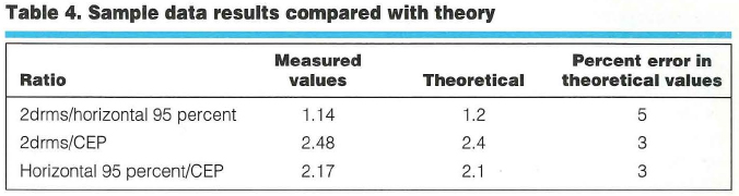
To evaluate Table 3’s efficacy, we used data from more than 550 hours (2 million data points) of differential GPS positions (DGPS), obtained with a U.S. Coast Guard reference station providing the differential corrections. Our results were 42 centimeters CEP, 91 centimeters horizontal 95 percent, and 104 centimeters 2drms. Table 4 shows how these results compare with Table 3’s theoretical values.
Data: Frank van Diggelen
Closing the Circle. The circular Gaussian distribution model for horizontal errors is surprisingly good. Figure 1 portrays a histogram (in green) generated from the DGPS data. These data have a horizontal rms value of 0.52 meter. Overlaid on the green histogram is a bar graph, showing the theoretical histogram that would be obtained from data that truly were circularly distributed and Gaussian and that had the same horizontal rms as the measured data. As the figure shows, the measured and theoretical distributions agree extremely well. We can obtain similarly good fits for vertical error distributions modeled as 1-D Gaussian.
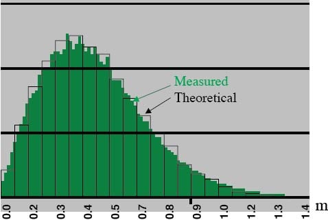
Figure 1. Measured and theoretical horizontal error distribution. The vertical axis indicates the relative frequency of errors occurring in each error interval. Horizontal axis values are rounded. (Data: Frank van Diggelen)
COMMON MISCONCEPTIONS
By now, one may feel that accuracy measures are rather simple to understand. Still, general discussions about GPS and GLONASS position accuracies frequently contain several misconceptions. Here’s our attempt to set the record straight.
Misconception Number 1 — rms precisely equals one sigma (1s or 1 standard deviation). Well, actually this is true, as long as the mean error is zero. With most GPS or GPS/GLONASS systems, the mean errors (over a sufficiently long time interval) are zero, or close to zero, and so rms may be considered essentially equivalent to one sigma.
Misconception Number 2 — 2drms means “two-dimensional rms.”In fact, 2drms usually stands for “twice distance rms,” in which the “distance” is measured in a 2-D space, the horizontal plane. Thus, 2drms is a very confusing abbreviation: It is a two-dimensional measure, but the “2d” usually stands for twice distance. (Some publications about navigation accuracies, notably those issued by the North Atlantic Treaty Organization, use the alternative meaning of “2d.” Thus, their “2drms” is exactly one-half of the usual measure.)
Misconception Number 3 — 2drms is exactly equivalent to a 95 percent probability level. This untrue belief stems from the fact that, for a 1-D Gaussian distribution, 95 percent of it lies inside an interval from 2s to +2s. However, 2drms is a measure for a 2-D distribution. The percentage of scatter lying within a circle with radius equal to 2drms depends on the distribution shape. For a circular distribution, the percentage of scatter inside a 2drms circle is 98 percent. The “Deriving the Equivalent Accuracies Table” sidebar shows this. As the scatter becomes more elliptical (with different error distributions for the two horizontal coordinates), it also becomes more one-dimensional, causing the percentage of elliptical distribution values inside a 2drms circle to tend toward 95 percent.
For GPS units, when the whole sky is visible above a 10-degree mask angle, scatter is approximately circular. Typically, distributions become very elliptical when HDOP gets large (much greater than 1). Thus, for any GPS receiver in any environment, the circle with a radius equal to 2drms contains between 95 and 98 percent of the scatter. When HDOP is low, the percentage is closer to 98 percent; when HDOP is high, it is closer to 95 percent.
Misconception Number 4 — rms is perfectly comparable with a 68 percent probability level. This is true for only 1-D Gaussian distributions. For 2-D or 3-D Gaussian distributions, the percentage of the values distributed inside a circle (or sphere), with a radius equal to the rms value, depends on distribution shape.
Misconception Number 5 — The error distribution really is Gaussian.We use the assumption that the error distribution is Gaussian for analytical purposes, and over time, one can show that a circular Gaussian distribution can model the errors very well (see Figure 1). However, certain errors may not have a Gaussian distribution:
- Stand-alone GPS errors are dominated by selective availability. Because this is an artificial error source, the errors it contributes are not always Gaussian.
- Stand-alone GPS/GLONASS errors show distributions that match Gaussian distributions quite well (to about 10 percent) over a time period of, say, several hours.
- Differential errors over a long time
display distributions that match Gaussian patterns to within a few percent. This is true for both code differential and carrier-phase differential (commonly referred to as real-time kinematic, or RTK). Differential errors over a short time produce scatter dominated by multipath, which is fairly constant over a few minutes, and, hence, the distribution is distinctly non-Gaussian.
IN CONCLUSION
As Disraeli also noted, “An investment in knowledge pays the best interest.” We hope that this brief note has proven to be a worthwhile “investment” to readers, shedding light on the sometimes murky subject of accuracy measures used in GPS and GLONASS positioning. With the simple information provided, you should be able to compute the positioning accuracy of a system in a variety of measures and also, contrary to the old adage, be able to compare “apple A” with “orange B.”
| Further Reading |
| For an introduction to the statistics of GPS accuracy measures, see |
|
| For an extended mathematical description of position errors, see |
|
| For positional error discussions from the war fighter’s perspective (but also relevant to noncombat applications), see |
|
|
| For an advanced discussion about the statistics of GPS positioning errors, see |
|
| Deriving the Equivalent Accuracies Table |
| The function invchisq (p,2) computes the square of a circle’s radius such that the sum of squares of two random variables, each with rms = 1s = 1, has a probability p of falling inside the circle. This function allows users to relate rms to probability for a two-dimensional circular distribution.Comments are shown in curly brackets “{}.” Table 3 (about equivalent accuracy) contains entries with resolution of only two digits. It is impossible, in general, to provide more precise ratios, because the three initial assumptions are averages over the whole world, and, thus, are good only to within a few percent of error in any particular region.rms (vertical) = 1.9 3 rms (horizontal) {using VDOP/HDOP = 1.9} (1,3) entry = 1/1.9 = 0.53 (1,5) entry = 2 3 0.53 = 1.1CEP = 50 percent circle {first solve for CEP = x 3 rms (horizontal), then use that result to derive other ratios} rms (horizontal) = (check)2 3 rms (linear) {assuming a circular distribution} R = sqrt(invchisq ( 0.5,2)) = 0.83 3 (check)2 => CEP = 0.83 3 (check)2 3 rms (linear) = 0.83 3 rms (horizontal) (2,3) entry = 1/0.83 = 1.2 CEP = x 3 rms (vertical) = x 3 rms (horizontal) 3 1.9 = 0.83 3 rms (horizontal) => x = 0.83/1.9 = 0.44 (1,2) entry = 0.44R95 = 95 percent circle {first solve for R95 = x 3 rms (horizontal), then use that result to derive other ratios] R = sqrt(invchisq (0.95,2)) = 1.73 3 (check)2 => R95 = 1.73 3 (check)2 3 rms (linear) = 1.73 3 rms (horizontal)(3,4) entry = 1.7R95 = x 3 rms (vertical) = x 3 rms (horizontal) 3 1.9 = 1.73 3 rms (horizontal) => x = 1.73/1.9 = 0.91 (1,4) entry = 0.91R95 = 1.73 3 rms (horizontal) = 1.73 3 CEP/0.83 (2,4) entry = 1.73/0.83 = 2.1 2drms = 2 3 rms (horizontal) {by definition} (3,5) entry = 22drms = x 3 CEP = x 3 0.83 3 rms (horizontal) = x 3 0.83 3 2drms/2 => x = 2/0.83 = 2.4 (2,5) entry = 2.42drms = x 3 R95 = x 3 1.73 3 rms (horizontal) = x 3 1.73 3 2drms/2 => x = 2/1.73 = 1.16 (4,5) entry = 1.2 rms (3-D) = 2.1 3 rms (horizontal) {using PDOP/HDOP = 2.1} = 2.1 3 2drms/2 = 2.1 3 rms (vertical)/1.9 rms (3-D) = x 3 CEP = x 3 0.83 3 (2,6) entry = 2.5 rms (3-D) = x 3 R95 = x 3 1.73 3 (4,6) entry = 1.2 SEP based on simulation: rms (horizontal) = (check)2; rms (vertical) = rms (horizontal) 3 1.9; SEP = 2.38 = 1.68 3 rms (horizontal) Other SEP ratios derived from the aforementioned ratios. |


Subscribe to GPS World
If you enjoyed this article, subscribe to GPS World to receive more articles just like it.


Excellent article!